Motivation

Cardiovascular disease (CVD), also known as Heart disease, is the leading cause of death in the United States [1]. As of 2018, CVD claims 163.6 deaths per 100,000 Americans [1] and continues to remain a global issue in both developed and developing countries. Improving the detection of heart disease can help greatly with treating its potential consequences. Early detection and awareness is especially important as it can increase the chances of a patient’s survival by up to 80% if the proper steps are taken [2]. Medical professionals currently examine symptoms and metrics such as blood pressure, blood sugar levels, cholesterol levels, and many more to make informed conclusions about whether a patient has heart disease. Our team’s goal is to achieve this detection process through the usage of supervised and unsupervised ML models, ultimately classifying patients with an efficacy that is difficult to attain through traditional means.

Methods

Heart disease detection is not a problem foreign to machine learning, but has room for further exploration by applying different models. Currently, the use of both Naive Bayes and Decision Trees have proved to be valid approaches to this problem [3] and our team aims to replicate and improve upon some of this success through similar methods. However, we also want to investigate the usage of unsupervised clustering techniques such as K-means, Hierarchical Clustering, and GMM as potential forms of detecting useful underlying patterns in the data. Additionally, our group will attempt to use a Random Forest as an alternative supervised approach. We believe that Random Forests could be a valid approach as it is similar to Decision Trees, which have already been shown to be successful, except with bagging and randomly choosing attributes while growing trees to limit overfitting.

Dataset

Background

The dataset we will be using for this project comes from the University of California, Irvine’s machine learning repository. It was made by the contributions of Dr. Andras Janosi, Dr. William Steinbrunn, Dr. Matthias Pfisterer, and Dr. Robery Detrano. Each individual gathered the data from their respective medical institutions located in Hungary, Switzerland, Long Beach, and Cleveland. The original dataset has total of 76 features but our project will focus solely on the Cleveland dataset which is composed of a 14 features, a subset of these 76 features. Within this Cleveland dataset, there are a total of 303 data points.

Features

1. age (in years)
2. sex (1 = male, 0 = female)
3. cp: chest pain type (0 = asymptomatic, 1 = non-anginal pain, 2 = atypical angina, 3 = typical angina)
4. trestbps: resting blood pressure (in mm Hg on admission to the hospital)
5. chol: serum cholesterol in mg/dl
6. fbs (fasting blood sugar > 120 mg/dl) (1 = true; 0 = false)
7. restecg: resting electrocardiographic results (0 = normal, 1 = having ST-T wave abnormality, 2 = showing probable or definite left ventricular hypertrophy by Estes’ criteria)
8. thalach: maximum heart rate achieved
9. exang: exercise induced angina (1 = yes, 0 = no)
10. oldpeak: ST depression induced by exercise relative to rest
11. slope: slope of the peark exercise ST segment
12. ca: number of major vessels (0-3) colored by flourosopy
13. thal (1 = normal; 2 = fixed defect; 3 = reversable defect)
14. target (1 = presence of Heart disease, 0 = no presence of heart disease)

Note that attribute 14, target, is the label of each datapoint in our dataset.

Let us visualize the distribution of each of our features:

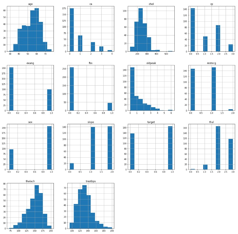
Looking at our data, we can see that the sex, cp, fbs, restecg, exang, slope, ca, and thal are categorical features while age, trestbps, chol, thalach, and oldpeak are continuous features. Additionally, the target feature is roughly uniformly distributed. This is ideal for supervised testing as it mitigates the situation where a model gets a high accuracy just from only classifiying the most probable label. When looking at the continuous features, the majority follow a somewhat normal distribution with the exception of the oldpeak feature.

Let us visualize the correlation between each of our features:

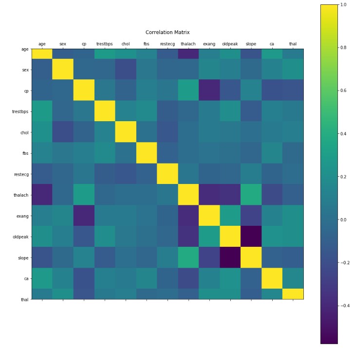
Looking at the correlation matrix, we can see that the majority of our features are relatively independent from one another. However, some relationships are notable. For example, the relationship between slope and oldpeak which shows a moderately negatively correlation. The realtionship between slope and thalach is moderately positively correlated. These relationships indicate that it may be possible to perform dimensional reduction on our data to reduce the amount of features and avoid the curse of dimensionality. Given that we will have 13 features after excluding the label, the curse of dimensionality may be an insignificant factor.

Unsupervised Approaches

Pre-Processing Data

Before we try clustering our dataset, it is important that we prepare our data points in order to increase our chances of success. Unfortunately, the majority of our features are categorical. Since a large portion of unsupervised methods utilize some sort of distance function to cluster data points, categorical features are often detrimental or irrelevant to it’s effectiveness. For example, category 0 is often no more different from category 1 than it is from category 2 but a distance function would interpret category 0 and 1 as more similar than category 0 and 2. Therefore, we remove the categorical features (sex, cp, fbs, restecg, exang, slope, ca, thal) from our dataset. This leaves us with 5 features (age, trestbps, chol, thalach, oldpeak) in our final data.

PCA

In order to perform dimensionality reduction, we will use PCA. In order to determine the amount of principle components we need, lets graph it against the recovered variance proportion:

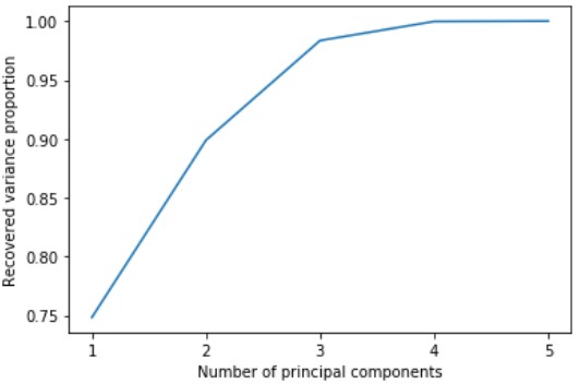
Looking at the graph, we can see that we can still get 99 % of the data’s variance using only 4 components. Therefore, we will reduce our data to its 4 principal components using PCA.

Ground Truth

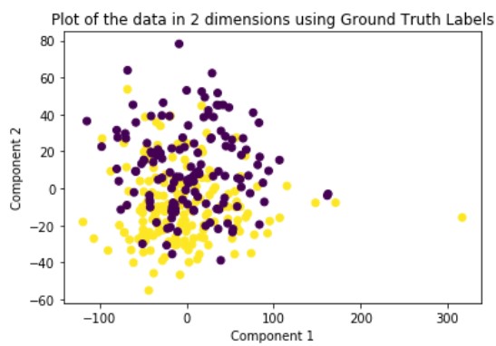
To help as a reference, we will plot the ground truth clustering based on the true labels of each data point. Note that in order to help visualize our clusters, we will plot using only the first two principle components but all the following methods will be assigning clusters based on their actual specified number of principle components.

K-Means

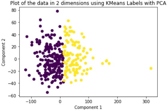
K-Means is a hard-assignment clustering method that requires you to specify the number of clusters you want beforehand. We set this number to two. The solution it outputs is a local solution and therefore is not guaranteed to be optimal. To solve for this problem, we run the method multiple times until we get a clustering with the best results. We run this method on the original data and the dimensionally reduced data.

Hierarchical Clustering

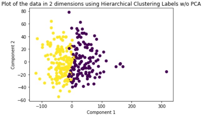
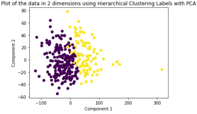
Hierarchical Clustering is a hard-assignment clustering method whose numbers of clusters is dependent upon what depth you decide to slice the created dendrogram. For our method, we are using agglomerative or bottom-up clustering to separate our data into two clusters. We run this method on the original data and the dimensionally reduced data.

GMM

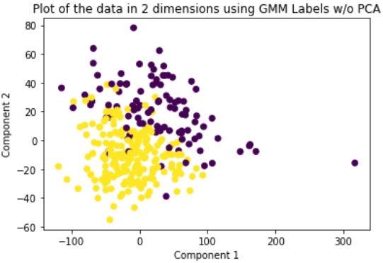
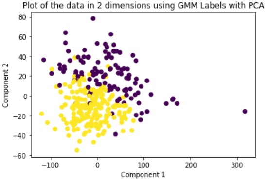
Gaussian Mixture Model or GMM is a soft-assignment clustering method. This means that for each data point, the model returns a probability of being in the cluster for each cluster. This is opposed to hard-assignment which assigns each data point to only a single cluster. GMM also requires the user to specify the number of clusters beforehand so we set this number to two. We run this method on the original data and the dimensionally reduced data.

Evaluation

In order to evaluate our clustering methods, we shall use four external measures. External measures evaluate the clustering based on the ground truth clustering. The measures we are using are the Fowlkes Mallows Score, V Measure, AMI, and the Adjusted Rand Index. The Fowlkes Mallows Score is a pairwise measure that ranges from 0 to 1 (higher score indicates a better clustering). V Measure is a matching-based measure that ranges from 0 to 1 (higher score indicates a better clustering). AMI(Adjusted Mutual Information) is an entropy-based measure that has an upper bound of 1 (higher score indicates a better clustering). The Adjusted Rand Index is a pairwise measure that ranges from -1 to 1 (higher score indicates a better clustering).

	Fowlkes Mallows Score	V Measure	AMI	Adjusted Rand Index
KMeans w/o PCA	0.5288	0.0138	0.0114	0.0205
Hierarchical Clustering w/o PCA	0.508	0.0111	0.0088	0.0133
GMM w/o PCA	0.5735	0.0698	0.0675	0.0948

	Fowlkes Mallows Score	V Measure	AMI	Adjusted Rand Index
KMeans with PCA	0.5288	0.0138	0.0114	0.0205
Hierarchical Clustering with PCA	0.5494	0.0272	0.0248	0.0395
GMM with PCA	0.576	0.0855	0.0832	0.1169

Looking at the results, we can see that clustering the dimensionally reduced data performed equal or better in every single metric for every single method. Between the methods, GMM performed the best in every metric. On the dimensionally reduced data, Hierarchical Clustering performed better than KMeans but the reverse is true on the data without using PCA. Overall, even based on GMM, the best performing method, the clustering did not achieve significant results given our binary clustering problem. We suspect that this could be because of multiple reasons. First, since the majority of our features were categorical and unsuitable for clustering, we lost a lot of meaningful information from our dataset that could have contributed to better clustering. Second, when looking at the plot of the ground truth labels, we can see that the labels aren’t well spatially separated. This separation may be clearer in higher dimensions but using only the first two principal components provides a good indication of the general trend of the data.

Supervised Approaches

Pre-Processing Data

Similar to what we did with the unsupervised approaches, it is important that we pre-process our dataset to increase our chances of success with our classifiers. Unlike unsupervised learning, categorical attributes can be valuable features in our dataset during training. However, we do still run into the problem of the difference between category 0 and category 1 being similar to the difference between category 0 and category 2. And yet, category 0 and category 1 are numerically closer. To solve this problem, we one-hot encode all of the category features. For example, instead of having a single feature with possible values (0, 1, 2), we separate it into three different features: is0, is1, and is2 with each feature being either true(1) or false(0). Additionally, we normalize our dataset so no features overpower others in our classifier. Our final dataset now has 30 features total. Given that we are going to use supervised approaches, lets split our data: 80% as our training data and 20% as our testing data.

PCA

In order to determine the amount of principal components we should use for dimensional reduction, lets plot this value against recovered variance proportion:

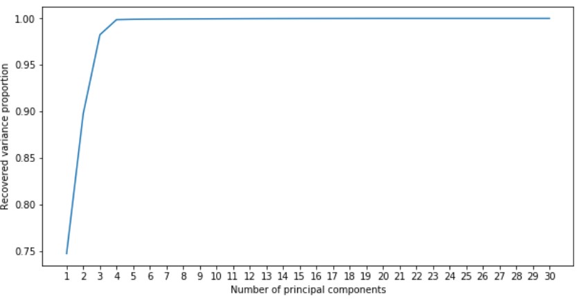
From this graph, we can see that with 4 principal components we still get 99% of datasets variance. Therefore, we will reduce our data to its 4 principal components.

Random Forest

Without PCA

In order to determine the value we should use for the number of estimators for our Random Forest Classifier, lets graph this value against the mean accuracy of our classifier on our testing data after being trained on our training data.

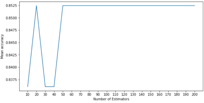
We can see that the mean accuracy plateaus after 50 estimators and so we will use that as the value of our hyper parameter. In order to evaluate our approach lets visualize the confusion matrix of our classifier.

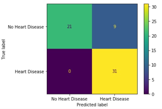
Looking at the confusion matrix, we can see that our random forest classifier performed fairly well. For our testing data, the method managed to correctly classify all of the patients with heart disease and approximately 2/3rds of those without heart disease.

With PCA

For the dimensionally reduced data, we will follow the same process as the original data.

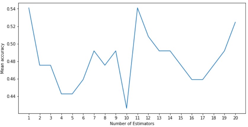
From this graph, we can see that the mean accuracy peaked at 1 and 11 estimators. We will use 11 as our hyper parameter.

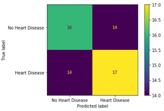
Looking at the confusion matrix, we can see that our random forest classifier performed fairly poorely. For both patients with and without heart disease, our classifier was only about 50% accurate: which is no better than just randomly guessing.

Evaluation

To evaluate our Random Forest Classifier, let us use Mean Accuracy and Root Mean Square Error (RMSE). For mean accuracy, higher is better but for RMSE, lower is better.

	Mean Accuracy	RMSE
Random Forest w/o PCA	0.8525	0.1475
Random Forest with PCA	0.541	0.459

Looking at our metrics, we can see that Random Forest on data w/o PCA is significantly more accurate than the data with PCA. We suspect that this is because when growing the trees for the classifier, having more attributes to potentially choose from allows the trees to capture more insight even if PCA maintains most of the data’s variance. Overall, our group believes that achieving 85.25% accuracy with our most successful Random Forest method is a result that is significantly accurate.

References

[1] J. Xu, S. Murphy, K. Kochanek, E. Arias, “Mortality in the United States”, 2018. NCHS Data Brief, no 355. Hyattsville, MD: National Center for Health Statistics. 2020.

[2] A. Åkesson, S. C. Larsson, A. Discacciati, and A. Wolk, “Low-Risk Diet and Lifestyle Habits in the Primary Prevention of Myocardial Infarction in Men,” Journal of the American College of Cardiology, vol. 64, no. 13, pp. 1299–1306, 2014.

[3] S. K. J. and G. S., “Prediction of Heart Disease Using Machine Learning Algorithms.,” 2019 1st International Conference on Innovations in Information and Communication Technology (ICIICT), CHENNAI, India, 2019, pp. 1-5.